Unlocking Multi-GPU Power for Lightning-Fast Image Embedding

Introduction

In the previous blog, I covered fine-tuning a CLIP model for Adobe Design UI icons to enhance searchability. Now, I scale up to generate embeddings using multiple GPUs, which presents several new challenges, particularly around optimizing efficiency in multi-GPU setups.

This blog explores these challenges, why they occur, and practical ways to optimize performance using a fine-tuned CLIP model to generate a large number of image vector embeddings. I'll share key insights into the performance gains, trade-offs, and the impact of different configurations.

Getting Started: Setting Up for Parallel Processing

Hardware Configuration:

• CPU: AMD EPYC™ 7282 - 16 Cores, 32 Threads @ 2.8 GHz
• Motherboard: ASRock Rack ROMED8-2T
• Memory: 128 GB ECC DDR4 @ 3200 MHz
• GPU: 4 x Nvidia RTX 3090 Founders Edition

Software Configuration:

• Python@3.12.7
• open_clip_torch@2.29.0
• torch@2.5.1
• Ubuntu@24.10

Line-by-Line Code Walkthrough

import open_clip
import os
import signal
import sys
import torch
import torch.distributed as dist
import time
 
from PIL import Image
from torch.utils.data import Dataset, DataLoader, DistributedSampler
from torch.distributed import Backend
 
 
# Define a custom dataset class for loading and preprocessing image data
class CustomImageDataset(Dataset):
    def __init__(self, img_data, preprocessor):
        self.img_data = img_data
        self.preprocessor = preprocessor
 
    def __len__(self):
        return len(self.img_data)
 
    def __getitem__(self, idx):
        image_path = self.img_data[idx].metadata["file_path"]
        image = Image.open(image_path)
        image = self.preprocessor(image)  # Apply the preprocessing steps
        return image  # Return the preprocessed image tensor
 
 
# Function to set up the PyTorch distributed environment
def setup_torch_distributed():
    # Initialize the process group for DDP using the NCCL backend, switch to GLOO if needed
    dist.init_process_group(backend=Backend.NCCL)
 
 
def main():
    # Enable faster convolutions by benchmarking the CUDA backend
    torch.backends.cudnn.benchmark = True
 
    # Setup the distributed environment for PyTorch
    setup_torch_distributed()
    
    # Retrieve the local rank of the current process (used for device assignment)
    local_rank = int(os.environ["LOCAL_RANK"])
    device = torch.device(f"cuda:{local_rank}")  # Assign the appropriate GPU to the process
 
    # Load the Vision Transformer (ViT) model and preprocessing function
    model, _, preprocess = open_clip.create_model_and_transforms(
        model_name="ViT-L-14",  # Specify the model name
        pretrained="/path/to/local/model.pt"  # Load a local fine-tuned model
    )
    model = model.to(device)  # Move the model to the appropriate GPU
    model.eval()  # Set the model to evaluation mode
 
    # Load the image metadata
    img_data = torch.load("image_docs.pt", weights_only=False)
    
    # Create a custom dataset and sampler for distributed data loading
    dataset = CustomImageDataset(img_data, preprocess)
    sampler = DistributedSampler(dataset)  # Ensures each process gets a unique subset of data
    dataloader = DataLoader(
        dataset=dataset,  # Pass the dataset to the DataLoader
        sampler=sampler,  # Use the distributed sampler
        batch_size=1080,  # Batch size (adjust based on GPU memory)
        pin_memory=True  # Optimizes data transfer between CPU and GPU
    )
 
    # Synchronize all processes to ensure they start at the same point, for benchmarking only
    dist.barrier(device_ids=[local_rank])
    start_time = time.time()
 
    # Generate embeddings without computing gradients (saves memory and speeds up computation)
    with torch.no_grad():
        for images in dataloader:  # Iterate through batches of images
            images = images.to(device, non_blocking=True)  # Move images to GPU
            embeddings = model.encode_image(images)  # Generate embeddings using the model
            # Further processing of embeddings can be added here if needed
 
    # Record the end time without additional synchronization
    total_seconds = time.time() - start_time
    print(f"Rank: {local_rank} with time: {total_seconds:.2f}s")
 
    # Clean up the distributed environment after successfully processing
    dist.destroy_process_group()
 
 
if __name__ == '__main__':
    main()
 

This code utilizes the PyTorch Distributed Data Parallel (aka DDP) module, typically used for model training, to perform parallel computation of image vector embeddings across multiple GPUs. The torchrun command, for example torchrun --nproc_per_node=2 src/icon_index_new.py, is used to efficiently manage the distributed processes, enabling the use of multiple GPUs for faster embedding generation.

Key Factors to Test for Enhanced Performance

In this section, we will assume that all these factors are tested with only a single GPU. Once we identify the optimized settings, these configurations will be used to scale up to 4 GPUs to evaluate performance improvements and scalability.

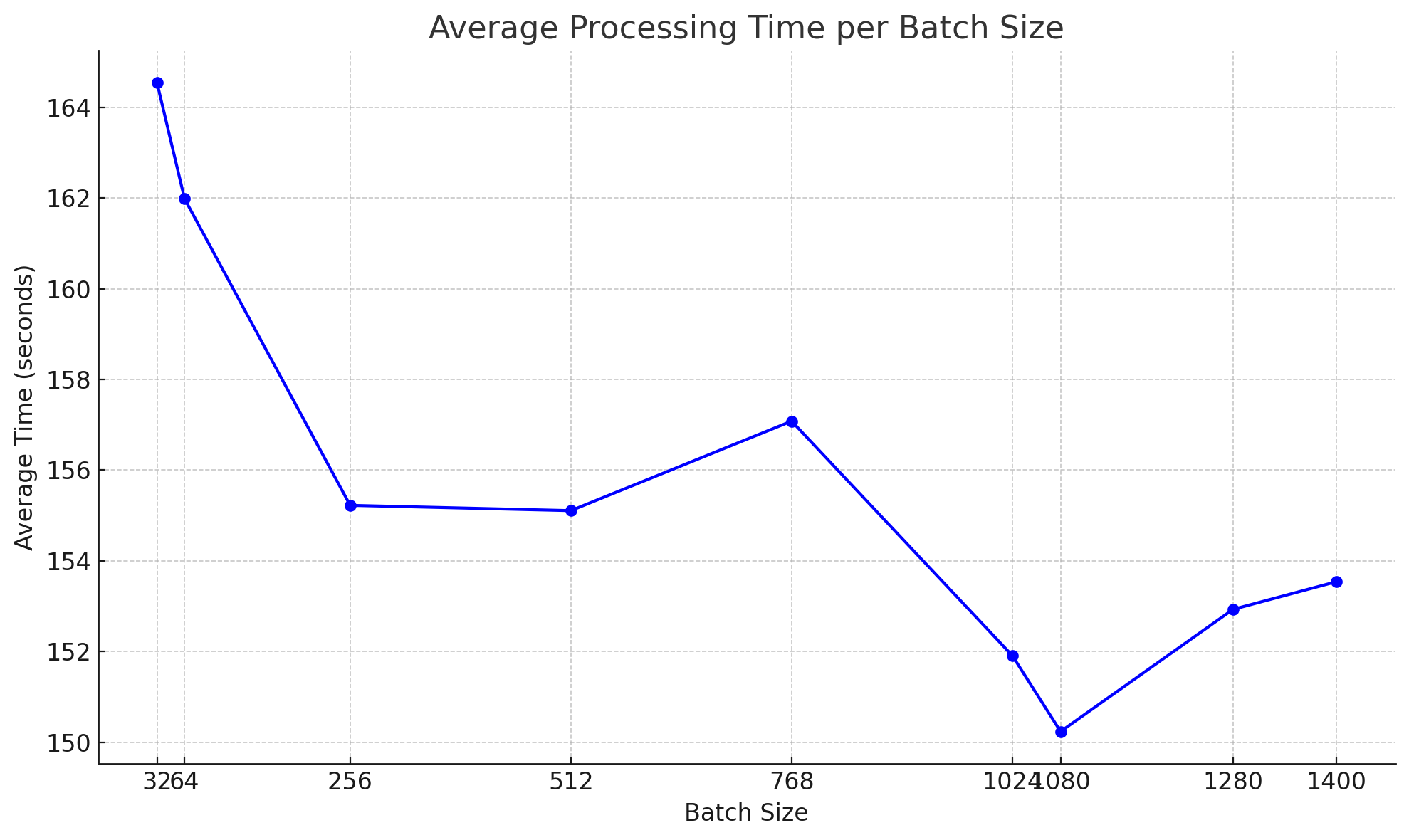
1. Batch Size: Trying different batch sizes helps improve GPU performance. Larger sizes reduce processing time until a point. The best batch size found was 1080, which was fastest without running out of memory. Sizes above 1280 had fewer benefits or caused memory issues.

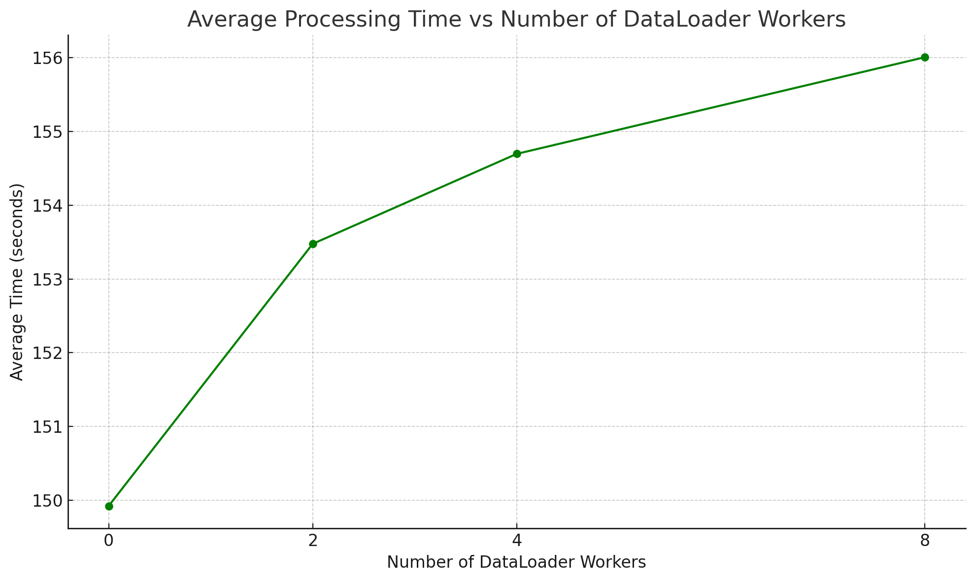
2. Number of DataLoader Workers: Testing num_workers showed that 0 had the best average time. Adding more workers (2, 4, 8) increased variability and provided no clear benefit.

3. Pin Memory: I tried pin_memory on and off but saw no performance difference. When true, it used a little bit more VRAM. See the When to set pin_memory to true? discussion for more details.

4. Distributed Backend (NCCL): I tested both NCCL and Gloo backends. No noticeable performance difference was observed. However, NCCL tends to spawn more Python processes to manage GPU-to-GPU communication efficiently.

5. Dataset Shuffling: I tested shuffling by turning it on and off. When shuffling was off, it was consistently slightly faster, but the performance difference was negligible. There was no significant memory consumption difference observed.

Analyzing Scalability: Does scale law apply to this scenario

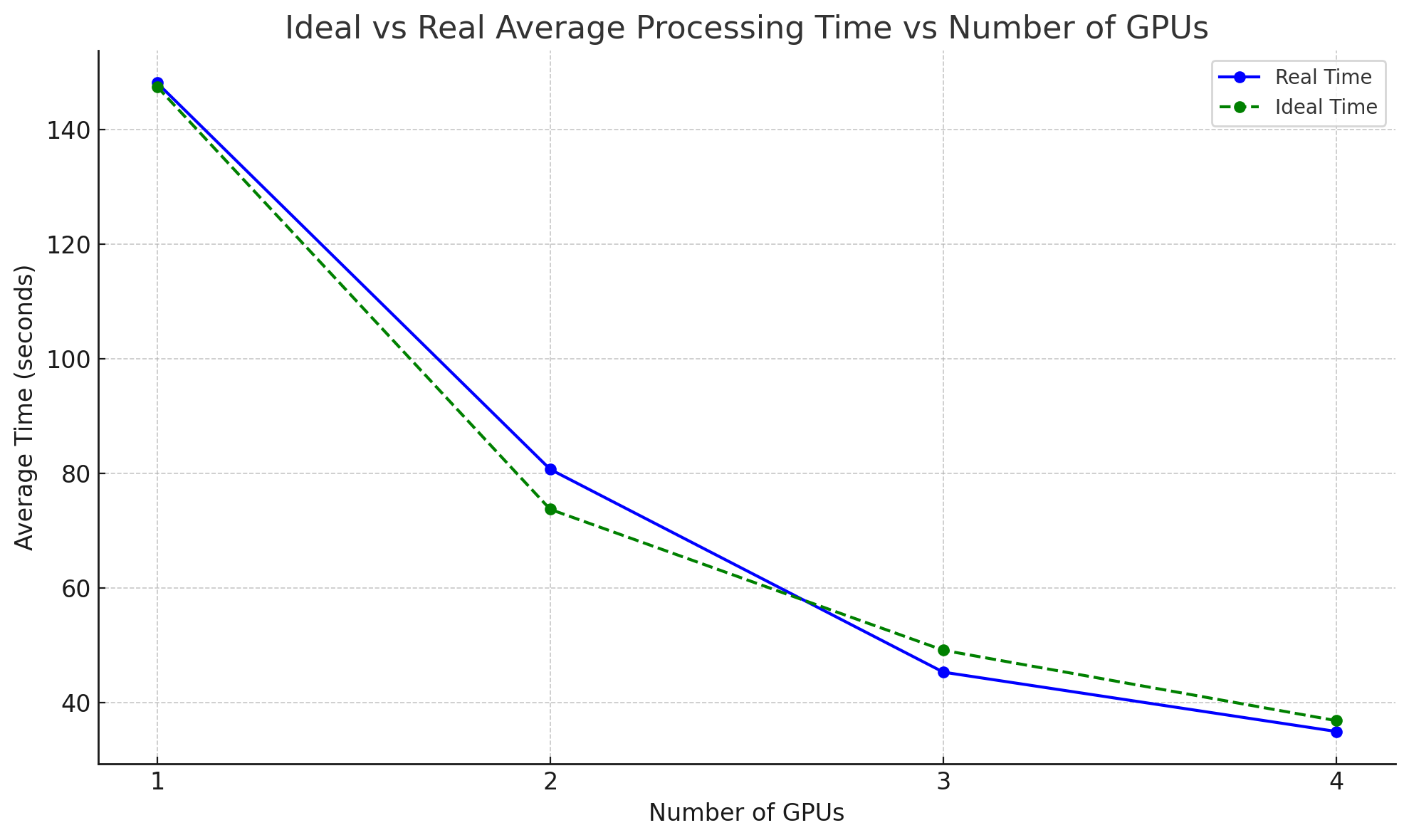
The scalability analysis was conducted by comparing the average processing time across different GPU counts, from 1 to 4 GPUs. The findings showed that as the number of GPUs increased, the processing time decreased. However, the reduction in time was not linear due to overheads such as GPU-to-GPU communication and synchronization. The observed time is even less than the ideal time, which would probably be due to the one GPU baseline performance error.

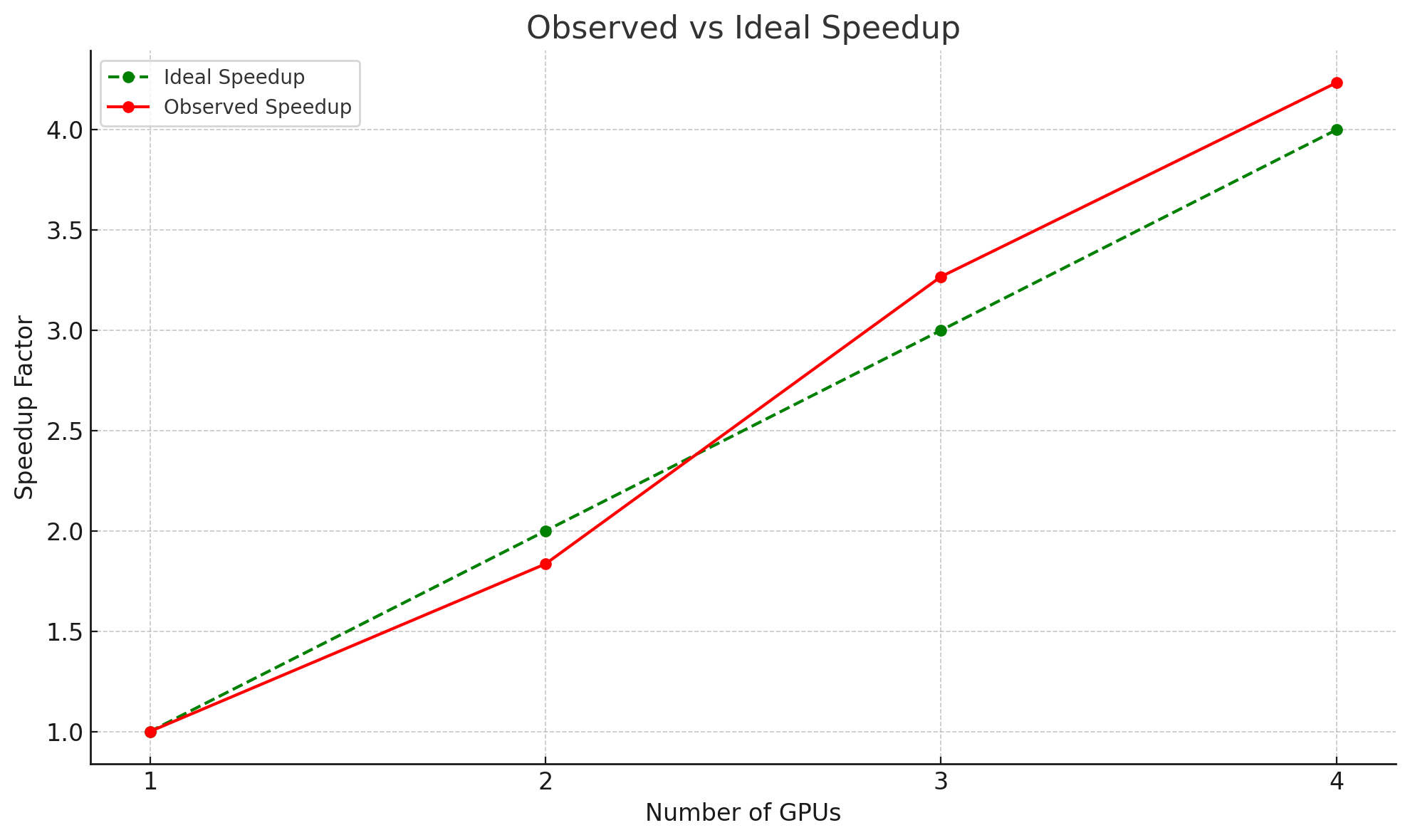
The speedup chart compared the ideal scenario—where each GPU would perfectly split the workload—with the observed performance. The ideal speedup showed a proportional reduction in time with more GPUs, while the real speedup demonstrated diminishing returns. This difference highlights the impact of practical challenges like synchronization delays and data transfer overheads, which prevent perfect scalability. The observed speedup outperformed the ideal speedup in three and four GPU scenarios, was probably due to the one GPU baseline performance error.

Also referenced Amdahl's Law and Gustafson's Law to understand the theoretical limits of parallelism and its effect on performance scaling in real-world scenarios.

• Amdahl's Law:

  $S = \dfrac{1}{(1 - P) + \dfrac{P}{N}}$

  Where:

  • S is the speedup of the system.
  • P is the proportion of the program that can be parallelized.
  • N is the number of processors (or GPUs).

  Amdahl's Law illustrates how the potential speedup of a process is limited by the proportion that must run serially. In simpler terms, even if you add more GPUs, the portion of work that can't be parallelized will limit the overall speedup.

• Gustafson's Law:

  $S = N - (1 - N) \times P$

  Where:

  • S is the speedup of the system.
  • P is the proportion of the program that can be parallelized.
  • N is the number of processors (or GPUs).

  Gustafson's Law suggests that as the problem size scales with more processors, the speedup is less constrained by the serial portion of the code. It provides a more optimistic view of scalability compared to Amdahl's Law, especially for large workloads.

Interesting Insights and Future Work

dist.barrier()

Using dist.barrier() in multi-GPU setups requires careful consideration to balance performance with resource usage. In this project, I used dist.barrier() to accurately measure the start time across all GPUs, ensuring synchronization. However, using NCCL as the distributed backend introduces extra costs, as Distributed Data Parallel (DDP) spawns $Num\_GPUs - 1$ additional Python processes to facilitate communication from GPU0 to other GPU devices. Each such process consumes approximately 256MB of VRAM. This can become a concern if VRAM is limited or if you are working with a large number of GPUs. It's important to be mindful of these potential costs when deciding whether or not to use dist.barrier().

For further reading, you can explore this Medium Blog, which explains why avoiding dist.barrier() might sometimes be beneficial, as well as these PyTorch discussion threads on why extra Python processes are spawned: Spawned Processes with DDP and `torch.distributed.barrier` used in multi-node distributed data-parallel.

Timing of Loading Tensor into GPU Device

During the tweaking of CustomImageDataset and DataLoader, I tested loading data to the device (GPU) in CustomImageDataset.__getitem__() versus in the main DataLoader loop. It turns out that the main loop option is far better. This approach is more efficient and increases performance because it processes data in batches. Loading data to the device in __getitem__() can also easily cause out-of-memory (OOM) errors.

Would NvLink Improve Performance?

I want to test it out